Calculating effect sizes

Load packages

require(gdata)
require(metafor)
require(dplyr)
require(ggplot2)

Download data

For this exercise, we’ll use the Curtis et al. (1999) data set that contains an array of plant measurements taken on 65 tree species under control and elevated CO₂ levels This data has been extracted from 84 papers and includes mean, standard deviation, coefficient of variation, and number of observations.

curtis<-read.xls("http://www.nceas.ucsb.edu/meta/Curtis/Curtis_CO2_database.xls",as.is=TRUE,verbose=FALSE,sheet=1)

str(curtis)

## 'data.frame':    784 obs. of  29 variables:
##  $ OBSNO   : int  1 2 3 4 5 6 7 8 9 10 ...
##  $ PAP_NO  : int  44 44 44 44 44 44 44 44 44 44 ...
##  $ PARAM   : chr  "PN" "PN" "AGWT" "AGWT" ...
##  $ P_UNIT  : chr  "umolCO2/m2/s" "umolCO2/m2/s" "mg" "mg" ...
##  $ GENUS   : chr  "ALNUS" "ALNUS" "ALNUS" "ALNUS" ...
##  $ SPECIES : chr  "RUBRA" "RUBRA" "RUBRA" "RUBRA" ...
##  $ DIV1    : chr  "WOODY" "WOODY" "WOODY" "WOODY" ...
##  $ DIV2    : chr  "N2FIX" "N2FIX" "N2FIX" "N2FIX" ...
##  $ AMBC    : num  350 350 350 350 350 350 350 350 350 350 ...
##  $ ELEV    : num  650 650 650 650 650 650 650 650 650 650 ...
##  $ CO2_UNIT: chr  "ul/l" "ul/l" "ul/l" "ul/l" ...
##  $ TIME    : int  46 46 47 47 47 47 47 47 47 47 ...
##  $ POT     : chr  "0.5" "0.5" "0.5" "0.5" ...
##  $ METHOD  : chr  "GC" "GC" "GC" "GC" ...
##  $ STOCK   : chr  "SEED" "SEED" "SEED" "SEED" ...
##  $ XTRT    : chr  "FERT" "FERT" "FERT" "FERT" ...
##  $ LEVEL   : chr  "HI" "CONTROL" "HI" "CONTROL" ...
##  $ QUANT   : chr  "20mgN/l" "." "20mgN/l" "." ...
##  $ SOURCE  : chr  "T3" "T3" "T1" "T1" ...
##  $ X_AMB   : num  11.8 11.7 2500.5 1460.5 1444.5 ...
##  $ SE_AMB  : num  0.64 1.16 324.3 76.6 219.6 ...
##  $ SD_AMB  : num  1.43 2.59 725.16 171.28 491.04 ...
##  $ CV._AMB : num  12.8 23.3 30.5 12.3 35.7 ...
##  $ N_AMB   : int  5 5 5 5 5 5 5 5 5 5 ...
##  $ X_ELEV  : num  23.2 25.9 4076.4 1805.3 2740.6 ...
##  $ SE_ELEV : num  4.61 1.48 601.7 221.1 525.2 ...
##  $ SD_ELEV : num  10.31 3.31 1042.17 494.39 909.67 ...
##  $ CV._ELEV: num  46.7 13.4 27.7 28.8 36 ...
##  $ N_ELEV  : int  5 5 3 5 3 5 3 5 3 5 ...

Please note that you may have to specify the location of the ‘perl interpreter’, e.g.

perl<-"http://www.nceas.ucsb.edu/meta/Curtis"
curtis<-read.xls("http://www.nceas.ucsb.edu/meta/Curtis/Curtis_CO2_database.xls",as.is=TRUE,verbose=FALSE,sheet=1,perl=perl)

Calculate effect sizes

For the Curtis data set, the response variables are all measured on a continuous scale. This allows us to calculate a number of traditional effect sizes, including Hedge’s D and the log-response ratio. In ‘metafor’ these effect sizes are referred to as ‘SMD’ and ‘ROM’, respectively.

In this case, we need the following variables to calculate effect sizes: mean, standard deviation, and sample size.

Additionally, sampling variances can be estimated differently. The default setting (used here) is the ‘large-sample approximation’ (vtype=’LS’). For Hedge’s D, one can also estimate ‘unbiased estimates’ (vtype=’UB’); for log-response ratio, ‘LS’ calculates sampling variance without assuming homoscedasticity while ‘HO’ assumes that variances are the same in control and treatment groups.

Note that ‘group 1’ (e.g. ‘m1i’ , ‘sd1i’) correspond to the treatment group and ‘group 2’ (e.g. ‘m2i’, ‘sd2i’) correspond to the control group.

Hedges’ D: Photosynthesis

curtis_ES<-escalc(measure='SMD', m2i=X_AMB , sd2i=SD_AMB, n2i=N_AMB, m1i=X_ELEV, sd1i=SD_ELEV, n1i=N_ELEV, vtype='LS',var.names=c("Hedges_D","Hedges_var"),data=curtis)

Visualize effect sizes (part I): forest plots

Please note that the first 25 observations are presented for visualization reasons. If you want to look at all effect sizes, use the name of the larger data frame (‘hedges_PN’) in the ‘forest’ function.

hedges_PN<-filter(curtis_ES, PARAM=="PN")
hedges_PN<-arrange(hedges_PN, GENUS)
hedges_PNN<-hedges_PN[1:25,]  # not necessary

forest(hedges_PNN$Hedges_D,hedges_PNN$Hedges_var, slab=hedges_PNN$GENUS, showweights=FALSE)

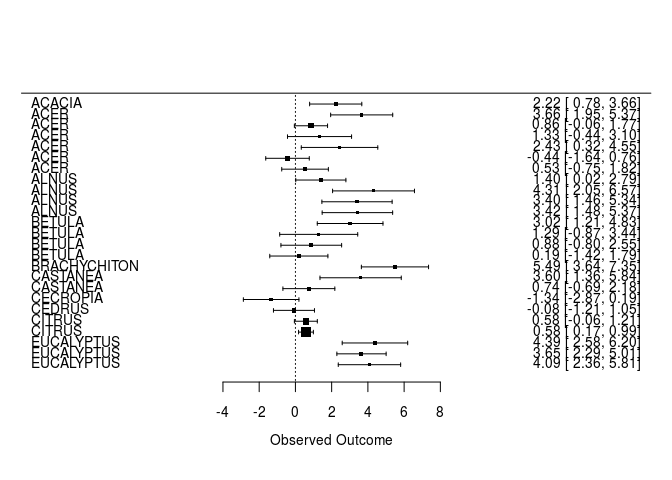
QUESTION: Do trees have higher or lower photosynthesis under ambient or elevated CO₂ conditions?

Visualize effect sizes (part II): explore moderators

Alternatives for visually assessing effect sizes (per group) include histograms or density distributions.

hedges_PN$SE<-sqrt(hedges_PN$Hedges_var)

dodge <- position_dodge(width=1)

ggplot(hedges_PN, aes(x=DIV2, y=Hedges_D, colour=DIV2)) + 
    geom_hline(yintercept=0,color="red")+
    #geom_errorbar(aes(ymin=Hedges_D-SE, ymax=Hedges_D+SE), width=.1,position=dodge) +
    geom_point(position=dodge)+ labs(x="Plant group", y="Effect size")+
     guides(fill=FALSE,colour=guide_legend(title="Plant group",title.position = "top"))+
  
  theme_bw()

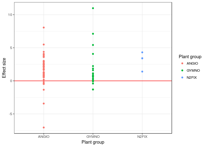
QUESTION: Are there differences among functional groups in terms of their response to elevated CO₂?#

LRR: water-use efficiency

The log-response ratio is a commonly used effect size and – once back-transformed – is easier to understand (e.g. the mean effect size is 10% greater than the control).

require(metafor,quietly = TRUE)

curtis_ES2<-escalc(measure='ROM', m2i=X_AMB , sd2i=SD_AMB, n2i=N_AMB, m1i=X_ELEV, sd1i=SD_ELEV, n1i=N_ELEV, vtype='LS',var.names=c("LRR","LRR_var"),data=curtis)

## Warning in log(m1i/m2i): NaNs produced

str(curtis_ES2)

## Classes 'escalc' and 'data.frame':   784 obs. of  31 variables:
##  $ OBSNO   : int  1 2 3 4 5 6 7 8 9 10 ...
##  $ PAP_NO  : int  44 44 44 44 44 44 44 44 44 44 ...
##  $ PARAM   : chr  "PN" "PN" "AGWT" "AGWT" ...
##  $ P_UNIT  : chr  "umolCO2/m2/s" "umolCO2/m2/s" "mg" "mg" ...
##  $ GENUS   : chr  "ALNUS" "ALNUS" "ALNUS" "ALNUS" ...
##  $ SPECIES : chr  "RUBRA" "RUBRA" "RUBRA" "RUBRA" ...
##  $ DIV1    : chr  "WOODY" "WOODY" "WOODY" "WOODY" ...
##  $ DIV2    : chr  "N2FIX" "N2FIX" "N2FIX" "N2FIX" ...
##  $ AMBC    : num  350 350 350 350 350 350 350 350 350 350 ...
##  $ ELEV    : num  650 650 650 650 650 650 650 650 650 650 ...
##  $ CO2_UNIT: chr  "ul/l" "ul/l" "ul/l" "ul/l" ...
##  $ TIME    : int  46 46 47 47 47 47 47 47 47 47 ...
##  $ POT     : chr  "0.5" "0.5" "0.5" "0.5" ...
##  $ METHOD  : chr  "GC" "GC" "GC" "GC" ...
##  $ STOCK   : chr  "SEED" "SEED" "SEED" "SEED" ...
##  $ XTRT    : chr  "FERT" "FERT" "FERT" "FERT" ...
##  $ LEVEL   : chr  "HI" "CONTROL" "HI" "CONTROL" ...
##  $ QUANT   : chr  "20mgN/l" "." "20mgN/l" "." ...
##  $ SOURCE  : chr  "T3" "T3" "T1" "T1" ...
##  $ X_AMB   : num  11.8 11.7 2500.5 1460.5 1444.5 ...
##  $ SE_AMB  : num  0.64 1.16 324.3 76.6 219.6 ...
##  $ SD_AMB  : num  1.43 2.59 725.16 171.28 491.04 ...
##  $ CV._AMB : num  12.8 23.3 30.5 12.3 35.7 ...
##  $ N_AMB   : int  5 5 5 5 5 5 5 5 5 5 ...
##  $ X_ELEV  : num  23.2 25.9 4076.4 1805.3 2740.6 ...
##  $ SE_ELEV : num  4.61 1.48 601.7 221.1 525.2 ...
##  $ SD_ELEV : num  10.31 3.31 1042.17 494.39 909.67 ...
##  $ CV._ELEV: num  46.7 13.4 27.7 28.8 36 ...
##  $ N_ELEV  : int  5 5 3 5 3 5 3 5 3 5 ...
##  $ LRR     : atomic  0.679 0.795 0.489 0.212 0.64 ...
##   ..- attr(*, "measure")= chr "ROM"
##   ..- attr(*, "ni")= int  10 10 8 10 8 10 8 10 8 10 ...
##  $ LRR_var : num  0.0424 0.0131 0.0386 0.0178 0.0598 ...
##  - attr(*, "digits")= num 4
##  - attr(*, "yi.names")= chr "LRR"
##  - attr(*, "vi.names")= chr "LRR_var"

Visualize effect sizes (part I) : forest plots

require(metafor,quietly = TRUE)
require(dplyr,quietly=TRUE)

LRR_WUE<-filter(curtis_ES2, PARAM=="WUE")
LRR_WUE<-arrange(LRR_WUE, GENUS)

forest(LRR_WUE$LRR,LRR_WUE$LRR_var, slab=LRR_WUE$GENUS, showweights=TRUE)

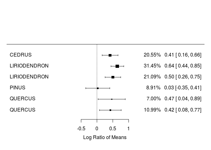
Note that the percentage next to each effect size is the weight of each point.

QUESTION: Do trees have higher or lower water-use efficiency in response to elevated CO₂?

Exercise: calculate effect sizes and create forest plots using the Stewart et al. bird abundance dataset

Download the dataset here
Review metadata for these datasets here and here