Confounding effects and extra tricks

Getting started

We’ll continue using the same data from previous days.

Load packages

require(gdata)
require(metafor)
require(dplyr)
require(compute.es)
require(ggplot2)
require(cowplot)
require(pez)
require(phytools)
require(ape)

Download data (Curtis et al. 1999)

curtis<-read.xls("http://www.nceas.ucsb.edu/meta/Curtis/Curtis_CO2_database.xls",as.is=TRUE,verbose=FALSE,sheet=1)
curtis_ES<-escalc(measure='ROM', m2i=X_AMB , sd2i=SD_AMB, n2i=N_AMB, m1i=X_ELEV, sd1i=SD_ELEV, n1i=N_ELEV, vtype='LS',var.names=c("LRR","LRR_var"),data=curtis)

## Warning in log(m1i/m2i): NaNs produced

#summary(as.factor(curtis_ES$PARAM))
curtis_WT<-filter(curtis_ES, PARAM=="TOTWT") # let's use whole plant weight because it has the largest number of observations   

curtis_WT$GEN_SPP<-paste(curtis_WT$GENUS,curtis_WT$SPECIES,sep="_")

Conversion among effect sizes

‘Compute.es’ is a powerful package that converts effect sizes.

The main function for calculating effect sizes is mes and des ,and res convert among effect sizes.

Here, we will first calculate basic effect sizes using mes and then convert the effect size r to Fisher’s z

# calculate effect sizes
curtis_ES<-mes(m.2=curtis_WT$X_AMB, m.1=curtis_WT$X_ELEV, sd.2=curtis_WT$SD_AMB, sd.1=curtis_WT$SD_ELEV, n.2=curtis_WT$N_AMB, n.1=curtis_WT$N_ELEV ,verbose=FALSE)


# convert correlation coefficient to fisher's z  
new_ES<-res(r=curtis_ES$r,var.r=curtis_ES$var.r, n=curtis_ES$N.total,verbose=FALSE)

curtis_ESS<-dplyr::select(new_ES, r, var.r, N.total, fisher.z, var.z)

head(curtis_ESS)

##       r var.r N.total fisher.z var.z
## 1  0.71  0.02       8     0.89  0.20
## 2  0.31  0.08      10     0.32  0.14
## 3  0.59  0.03      10     0.68  0.14
## 4 -0.21  0.09      10    -0.21  0.14
## 5  0.19  0.11       8     0.19  0.20
## 6  0.81  0.01       8     1.13  0.20

r_z<-ggplot(curtis_ESS, aes(x=r, y=fisher.z))+geom_point() +
  
    geom_abline(intercept = 0, slope = 1,colour="red")+theme_bw()

r_z

hist_r<-ggplot(curtis_ESS, aes(r)) +
  geom_density(colour="red")+xlab("r")+theme_bw()


hist_z<-ggplot(curtis_ESS, aes(fisher.z)) +
  geom_density(color="blue")+xlab("Fisher's Z")+theme_bw()

ab<-plot_grid(hist_r, hist_z, ncol=2)
ab

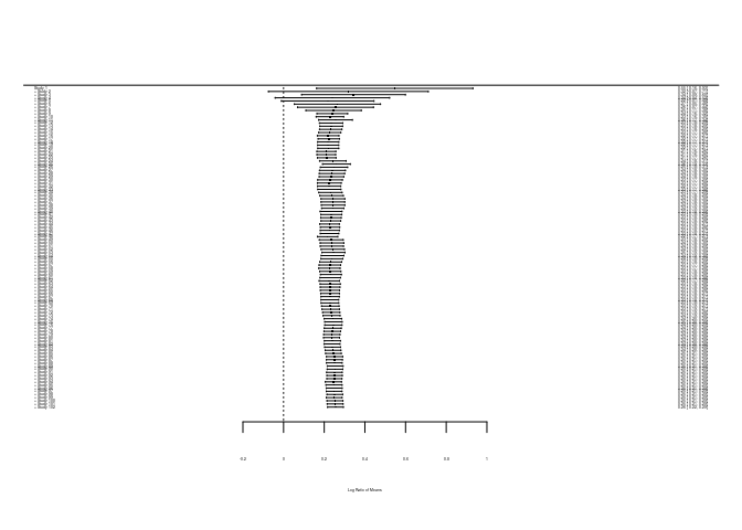
Cumulative meta-analysis

This method tests whether effect sizes have shifted over time. It fits the model by iteratively adding observations in the order that we designate.

re_wt<-rma(LRR, LRR_var, data=curtis_WT)

cum_re<-cumul(re_wt, order(curtis_WT$OBSNO))

forest.cumul.rma(cum_re)

Controlling for shared evolutionary history (phylogeny)

For species-level analyses, shared evolutionary history should be controlled for above and beyond random effect terms already included.

Clean data set

The basic steps are:

Resolve taxonomic names to ensure that as many as possible can be placed on a phylogeny.
Build phylogeny. If you’re interested in how to build a phylogeny, here’s the code
Make sure that your phylogeny has the same number of tip labels as there are species in the data set.

setwd('/homes/dc78cahe/Dropbox (iDiv)/Teaching/MetaAnalysis_Course/pages/Day4_files/')
clean<-read.csv("TPL_sppnames.csv")
clean<-dplyr::select(clean,GEN_SPP2=Taxon, phy=new_species)
clean$GEN_SPP2<-as.character(clean$GEN_SPP2)

curtis_WT$GENUS<-tolower(as.character(curtis_WT$GENUS))
curtis_WT$GENUS<-paste(toupper(substr(curtis_WT$GENUS, 1, 1)), substr(curtis_WT$GENUS, 2, nchar(curtis_WT$GENUS)), sep="")

curtis_WT$SPECIES<-tolower(as.character(curtis_WT$SPECIES))
curtis_WT$GEN_SPP2<-as.character(paste(curtis_WT$GENUS, curtis_WT$SPECIES,sep=" "))

curtis_WT$GEN_SPP2<-ifelse(curtis_WT$GEN_SPP2=="Populusx euramericana","Populus × euramericana",curtis_WT$GEN_SPP2)

curtis_WT<-dplyr::left_join(curtis_WT,clean, by="GEN_SPP2")

# read in tree

tree<-read.tree("Curtis_phylogeny.tre")
str(tree)

## List of 5
##  $ edge       : int [1:68, 1:2] 36 37 37 38 39 39 40 40 38 41 ...
##  $ Nnode      : int 34
##  $ tip.label  : chr [1:35] "Pseudotsuga_menziesii" "Picea_glauca" "Picea_mariana" "Picea_abies" ...
##  $ edge.length: num [1:68] 144.6 207.6 23.1 100.8 83.7 ...
##  $ node.label : chr [1:34] "Spermatophyta" "" "" "" ...
##  - attr(*, "class")= chr "phylo"
##  - attr(*, "order")= chr "cladewise"

# we need to drop one species from our data frame ('Trichospermum mexicanum' because it wasn't placed on the phylogeny)

curtis_WTT<-filter(curtis_WT, phy!="Trichospermum_mexicanum")

length(unique(curtis_WTT$phy))

## [1] 35

#same number of species on phylogeny as in data set?

length(unique(curtis_WTT$phy))==length(unique(tree$tip.label))

## [1] TRUE

Fit multi-level meta-analytical model that accounts for shared phylogenetic history

Make a phylogenetic correlation matrix
Fit model such that there is a random term for species, which is then matched to a correlation matrix (‘R’)
Compare it to a model that doesn’t account for phylogeny

tree_m<-vcv.phylo(tree, cor=TRUE) # creates phylogenetic correlation matrix

re_phy<-rma.mv(LRR, LRR_var, mods=~1,random=list(~1|PAP_NO, ~1|XTRT, ~1|phy), R=list(phy=tree_m), data=curtis_WTT)
summary(re_phy)

## 
## Multivariate Meta-Analysis Model (k = 101; method: REML)
## 
##   logLik  Deviance       AIC       BIC      AICc  
## -22.7040   45.4080   53.4080   63.8287   53.8291  
## 
## Variance Components: 
## 
##             estim    sqrt  nlvls  fixed  factor    R
## sigma^2.1  0.0124  0.1115     29     no  PAP_NO   no
## sigma^2.2  0.0080  0.0895      8     no    XTRT   no
## sigma^2.3  0.0088  0.0936     35     no     phy  yes
## 
## Test for Heterogeneity: 
## Q(df = 100) = 768.9932, p-val < .0001
## 
## Model Results:
## 
## estimate      se    zval    pval   ci.lb   ci.ub     
##   0.2745  0.0693  3.9597  <.0001  0.1386  0.4103  ***
## 
## ---
## Signif. codes:  0 '***' 0.001 '**' 0.01 '*' 0.05 '.' 0.1 ' ' 1

#
re_nophy<-rma.mv(LRR, LRR_var, mods=~1,random=list(~1|PAP_NO, ~1|XTRT, ~1|phy), data=curtis_WTT)
summary(re_nophy)

## 
## Multivariate Meta-Analysis Model (k = 101; method: REML)
## 
##   logLik  Deviance       AIC       BIC      AICc  
## -20.4116   40.8232   48.8232   59.2439   49.2443  
## 
## Variance Components: 
## 
##             estim    sqrt  nlvls  fixed  factor
## sigma^2.1  0.0087  0.0933     29     no  PAP_NO
## sigma^2.2  0.0094  0.0969      8     no    XTRT
## sigma^2.3  0.0042  0.0645     35     no     phy
## 
## Test for Heterogeneity: 
## Q(df = 100) = 768.9932, p-val < .0001
## 
## Model Results:
## 
## estimate      se    zval    pval   ci.lb   ci.ub     
##   0.2742  0.0455  6.0271  <.0001  0.1850  0.3634  ***
## 
## ---
## Signif. codes:  0 '***' 0.001 '**' 0.01 '*' 0.05 '.' 0.1 ' ' 1

Accountring for phylogeny, in this particular case, did not alter the mean effect size. However, the confidence intervals around the mean effect size are wider when accounting for phylogeny.

Exercise: do your own meta-analysis (using either Gibson et al. or another data set of your own choosing)

Tasks

Download data from Gibson et al.
Calculate effect sizes
Fit multi-levelr andom effects model
Make visualisations of your results (effect sizes, forest plot, etc.)